Calculate silhouette widths index for various numbers of partitions

Computes silhouette widths index for several possible numbers of clusters(partitions) k, which determines how well an object falls within their cluster compared to other clusters. The best number of clusters k is the one with the highest silhouette width.

Usage

get_sil_widths(dist_mat, max.k = 10)

# S3 method for sil_width_df
plot(x, ...)

Arguments

dist_mat: A Gower distance matrix, the output of a call to get_gower_dist.
max.k: The maximum number of clusters(partitions) to search across.
x: A sil_width_df object; the output of a call to get_sil_widths().
...: Further arguments passed to ggplot2::geom_line to control the appearance of the plot.

Details

get_sil_widths calls cluster::pam on the supplied Gower distance matrix with each number of clusters (partitions) up to max.k and stores the average silhouette widths across the clustered characters. When plot = TRUE, a plot of the sillhouette widths against the number of clusters is produced, though this can also be produced seperately on the resulting data frame using plot.sil_width_df(). The number of clusters with the greatest silhouette width should be selected for use in the final clustering specification.

Value

For get_sil_widths(), it produces a data frame, inheriting from class "sil_width_df", with two columns: k is the number of clusters, and sil_width is the silhouette widths for each number of clusters. If plot = TRUE, the output is returned invisibly.

For plot() on a get_sil_widths() object, it produces a ggplot object that can be manipulated using ggplot2 syntax (e.g., to change the theme or labels).

Examples

# See vignette("char-part") for how to use this
# function as part of an analysis pipeline

data("characters")

#Reading example file as categorical data
Dmatrix <- get_gower_dist(characters)

#Get silhouette widths for k=7
sw <- get_sil_widths(Dmatrix, max.k = 7)

sw
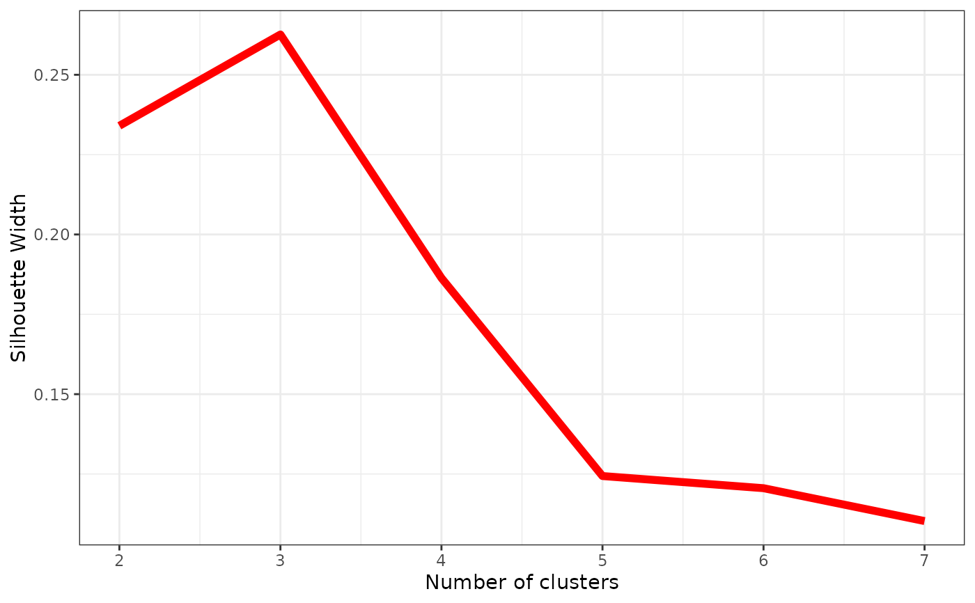
#>   k sil_width
#> 1 2 0.2340255
#> 2 3 0.2626128
#> 3 4 0.1863738
#> 4 5 0.1243595
#> 5 6 0.1205568
#> 6 7 0.1102649

plot(sw, color = "red", size =2)