This vignette explains how to conduct automated morphological character partitioning as a pre-processing step for clock (time-calibrated) Bayesian phylogenetic analysis of morphological data, as introduced by Simões and Pierce (2021).
Character Partitioning (Case 1)
Load the EvoPhylo package
1. Generate distance matrix
Generate a Gower distance matrix with get_gower_dist()
by supplying the file path of a .nex file containing a character data
matrix:
#Load a character data matrix from your local directory to produce a Gower distance matrix
dist_matrix <- get_gower_dist("DataMatrix.nex", numeric = FALSE)
## OR
#Load an example data matrix 'DataMatrix.nex' that accompanies `EvoPhylo`.
DataMatrix <- system.file("extdata", "DataMatrix.nex", package = "EvoPhylo")
dist_matrix <- get_gower_dist(DataMatrix, numeric = FALSE)
Below, we use the example data matrix characters that
accompanies EvoPhylo.
data(characters)

dist_matrix <- get_gower_dist(characters, numeric = FALSE)
2. Estimate the optimal number of partitions
The optimal number of partitions (clusters) will be first determined
using partitioning around medoids (PAM) with Silhouette widths index
(Si) using get_sil_widths(). The latter will estimate the
quality of each PAM cluster proposal relative to other potential
clusters.
## Estimate and plot number of cluster against silhouette width
sw <- get_sil_widths(dist_matrix, max.k = 10)
plot(sw, color = "blue", size = 1)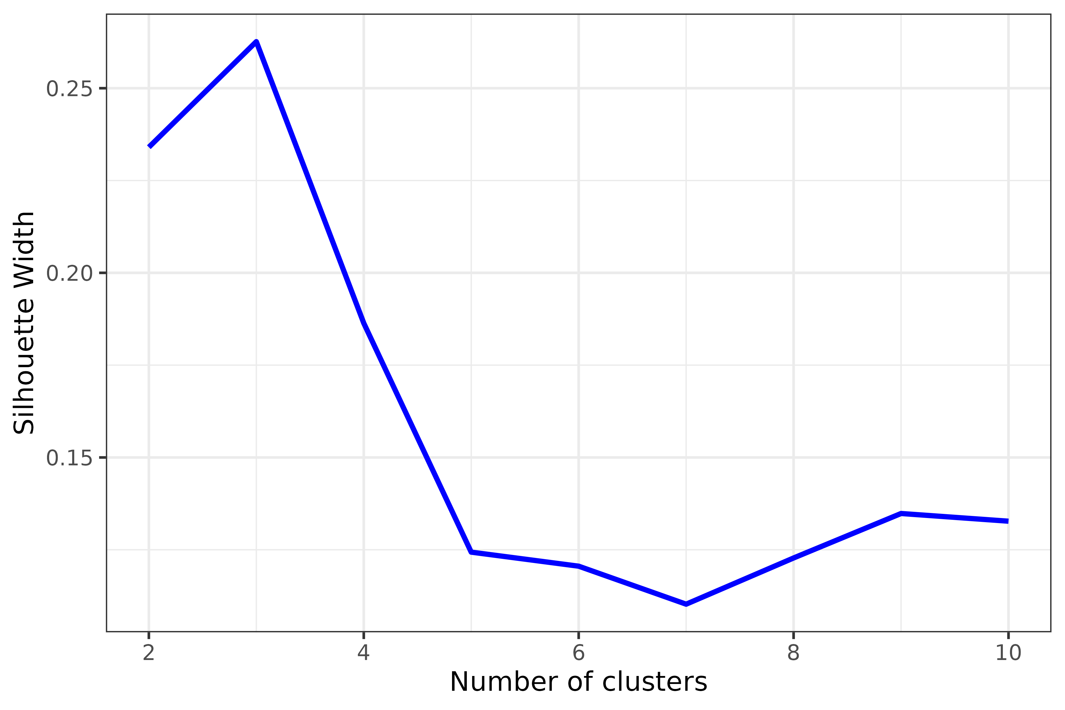
Decide on number of clusters based on plot; here, partitions appears optimal.
3. Simple Workflow
3.1. Analyze clusters with PAM under chosen
value (from Si) with make_clusters().
3.2. Produce simple cluster graph
3.3. Export clusters/partitions to Nexus file with
cluster_to_nexus() or
write_partitioned_alignments().
## Generate and vizualize clusters with PAM under chosen k value.
clusters <- make_clusters(dist_matrix, k = 3)

plot(clusters)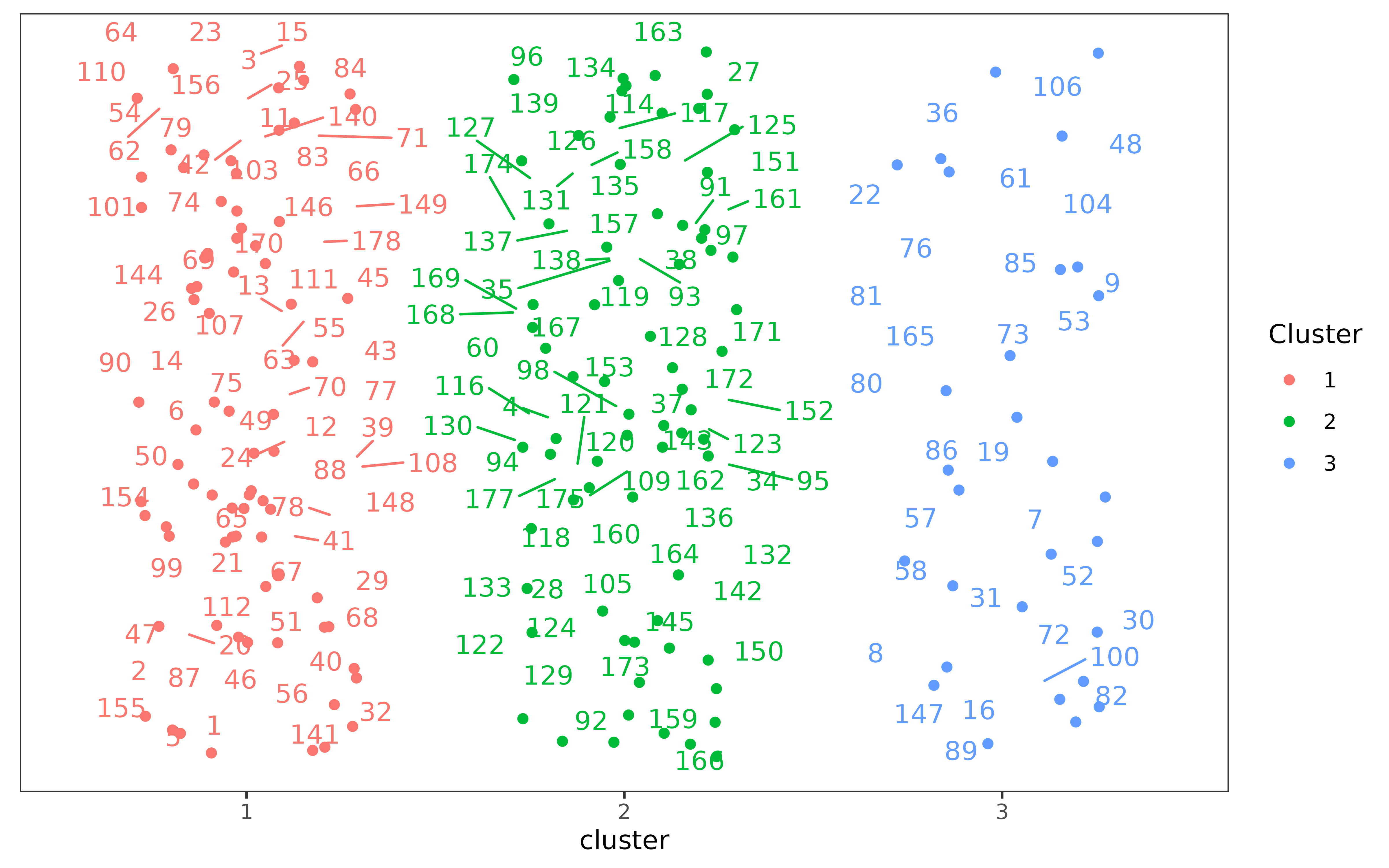
## Write clusters to Nexus file for Mr. Bayes
cluster_to_nexus(clusters, file = "Clusters_MB.txt")

## Write partitioned alignments to separate Nexus files for BEAUTi
# Make reference to your original character data matrix in your local directory
write_partitioned_alignments("DataMatrix.nex", clusters, file = "Clusters_BEAUTi.nex")
4. Complete Workflow
4.1. Analyze clusters with PAM under chosen
value (from Si) with make_clusters().
4.2. Produce a graphic clustering (tSNEs), coloring data points
according to PAM clusters, to independently verify PAM clustering. This
is set with the tsne argument within
make_clusters().
4.3. Export clusters/partitions to Nexus file with
cluster_to_nexus(). This can be copied and pasted into the
Mr. Bayes command
block. Alternatively, write the partitioned alignments as separate Nexus
files using write_partitioned_alignments(). This will allow
you to import the partitions separately into BEAUti for analyses with BEAST2.
#User may also generate clusters with PAM and produce a graphic clustering (tSNEs)
clusters <- make_clusters(dist_matrix, k = 3, tsne = TRUE, tsne_dim = 3)

plot(clusters, nrow = 2, max.overlaps = 5)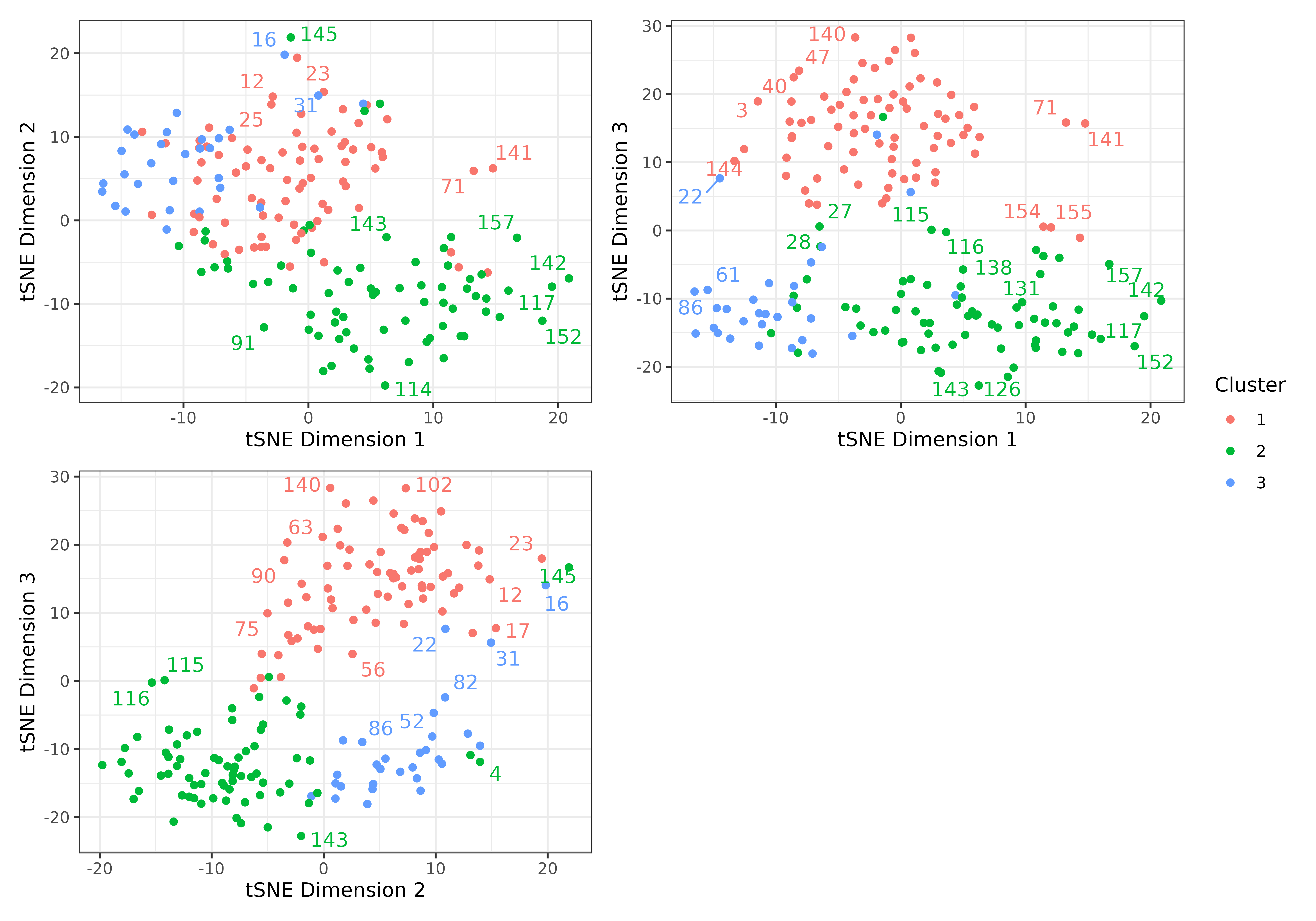
## Write clusters to Nexus file for Mr. Bayes
cluster_to_nexus(clusters, file = "Clusters_MB.txt")

## Write partitioned alignments to separate Nexus files for BEAUTi
# Make reference to your original character data matrix in your local directory
write_partitioned_alignments("DataMatrix.nex", clusters, file = "Clusters_BEAUTi.nex")
Character Partitioning (Case 2)
Here is an additional example of how to conduct automated morphological character partitioning. In this example, we utilize a combined evidence dataset (morphological and molecular data) of fossil and extant penguins from Ksepka et al. (2012), following similar modifications to this dataset as used in Gavryushkina et al. (2017) (removing all invariant characters from the dataset and all non-penguin taxa), resulting in 55 taxa and 201 characters for the morphological partition. A key feature of this dataset is the high amount of missing data in the fossil species. Therefore, it is recommended in such cases to reduce the number of observations with missing data (e.g. more than 30% of missing data, Ciampaglio, Kemp, and McShea (2001)). In this case, all fossils have more than 30% of missing data, and so only data from extant taxa were used to calculate character partitions.
1. Generate distance matrix
Generate a Gower distance matrix with get_gower_dist()
by supplying the file path of a .nex file containing a character data
matrix:
#Load a character data matrix from your local directory to produce a Gower distance matrix
dist_matrix <- get_gower_dist("Penguins_Morpho(VarCh)_Extant.nex", numeric = FALSE)
Or, for this example simply load the data matrix
‘Penguins_Morpho(VarCh)_Extant.nex’ that accompanies
EvoPhylo.
DataMatrix <- system.file("extdata", "Penguins_Morpho(VarCh)_Extant.nex", package = "EvoPhylo")
dist_matrix <- get_gower_dist(DataMatrix, numeric = FALSE)
2. Estimate the optimal number of partitions
The optimal number of partitions (clusters) will be first determined
using partitioning around medoids (PAM) with Silhouette widths index
(Si) using get_sil_widths(). The latter will estimate the
quality of each PAM cluster proposal relative to other potential
clusters.
## Estimate and plot number of cluster against silhouette width
sw <- get_sil_widths(dist_matrix, max.k = 10)
plot(sw, color = "blue", size = 1)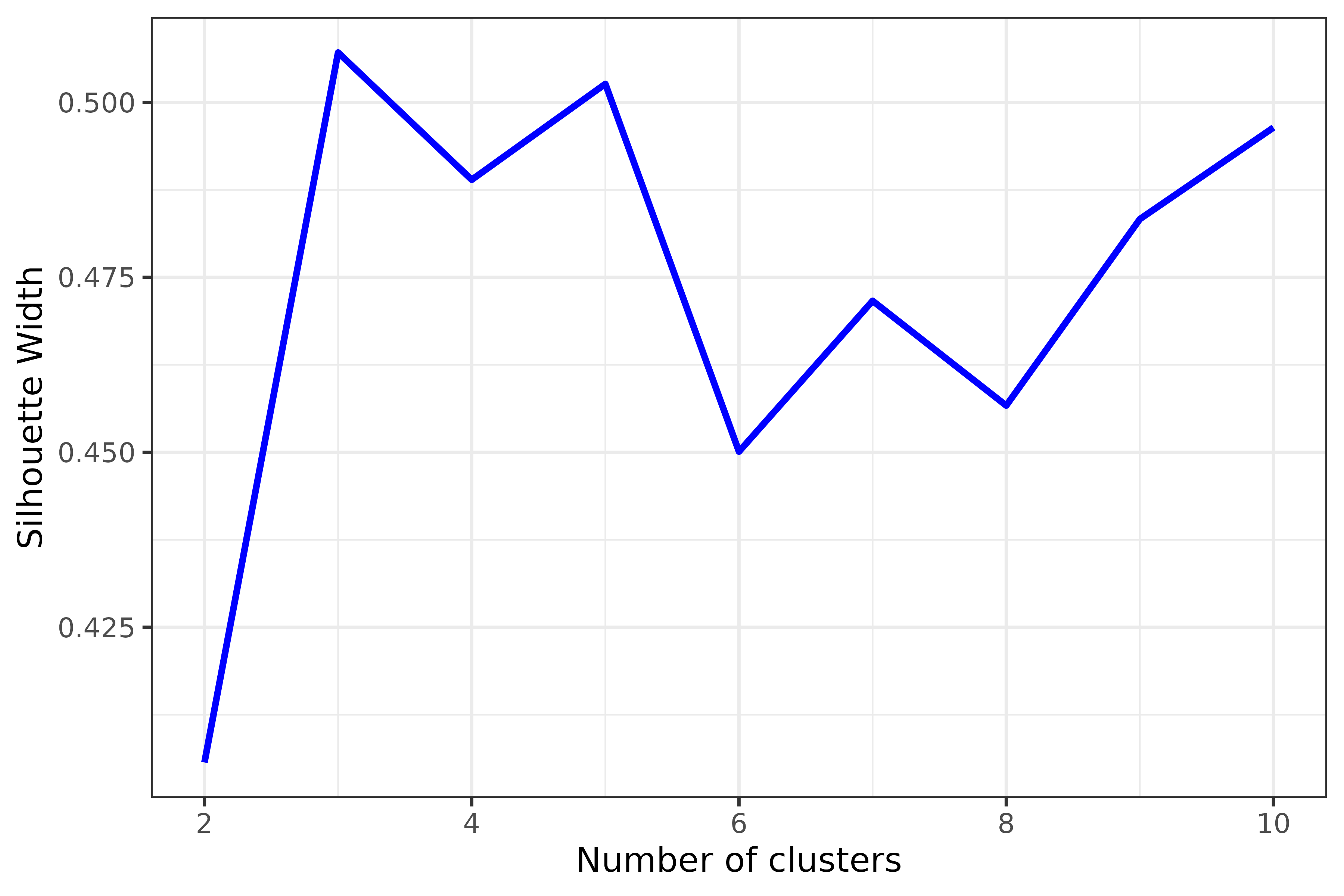
Decide on number of clusters based on plot; here, partitions appears optimal, Firstly followed by five partitions. In such cases, we encourage users to explore both number of partitions as the suboptimal partitioning (five) is close to the optimal number suggested (three). Deciding upon the final partitioning scheme shall be based on which number of partitions provides the best agreements between the first (PAM) and second (tSNEs) tests, or agreement with external evidence (anatomical or developmental subdivisions). For simplicity, here we explore only the option with three partitions.
3. Complete Workflow
3.1. Analyze clusters with PAM under chosen
value (from Si) with make_clusters().
3.2. Produce a graphic clustering (tSNEs), coloring data points
according to PAM clusters, to independently verify PAM clustering. This
is set with the tsne argument within
make_clusters().
3.3. In this example we will analyze this dataset with BEAST2, so we
will export the partitioned alignments as separate Nexus files using
write_partitioned_alignments(). This will allow you to
import the partitions separately into BEAUti for analyses with BEAST2. Remember to indicate the name
of the full data matrix file to be partitioned (including all extant and
fossil species in this case). The file name chosen
(“Penguins_Morpho_3p.nex”) will be automatically appended with
“…part
#User may also generate clusters with PAM and produce a graphic clustering (tSNEs)
clusters <- make_clusters(dist_matrix, k = 3, tsne = TRUE, tsne_dim = 3)

plot(clusters, nrow = 2, max.overlaps = 5)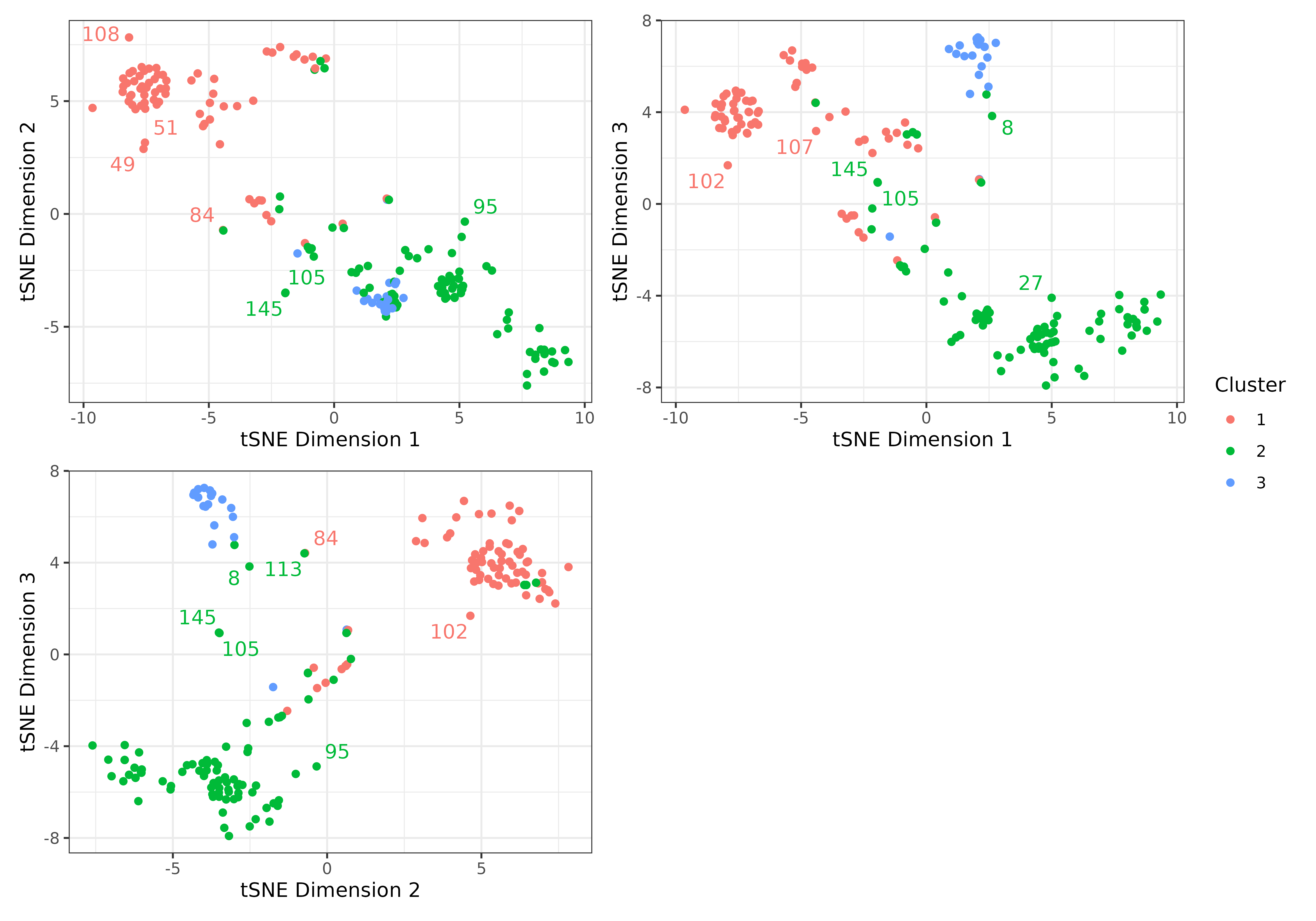
## Write partitioned alignments to separate Nexus files for BEAUTi
# Make reference to your original character data matrix in your local directory
write_partitioned_alignments("Penguins_Morpho(VarCha).nex", clusters, file = "Penguins_Morpho_3p.nex")